This page covers the steps used to visualize the gaussian cube files created in example 1 in Density Plot. This example uses VMD 1.9.2 but should be nearly the same for older versions.
It is useful to carry out this example to first familiarize yourself with VMD.
The following links allow you to download the files uesed and created in the example. Note that these files can be downloaded in-line with the descriptions below.
test_5.0_equalweights_complete.cube
test_5.0_equalweights_segment_1_region_1.cube
test_5.0_equalweights_segment_1_region_2.cube
From "File" chose "New Molecule" and load the test_5.0_equalweights_complete.cube file.
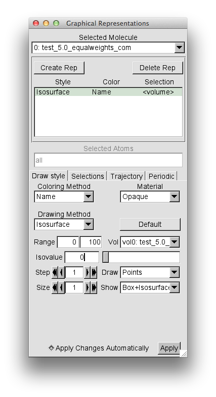
After loading, open the "Graphical Reprentations" widget from "Reprentations" selection in the "Graphics" pull-down tab. Then, for the "Drawing Method" option choose "Isosurface". This should give you the following window.
Note that the default settings are to Draw "Points" and Show "Box+Isosurface". Change these settings to "Wireframe" and "Isosurface" respectively.
Then change the "Isovalue" from the default 0 to 0.01 and press return. This is a reasonalbly low value to capture the complete volumetric data set.
Note: When loading multiple gaussian cube files, as shown below, make sure that the "Isovalue" setting is the same for all files, otherwise the visulaization may be misleading.
Then change the "Coloring Method" to "Color ID" and select 0 as the option.
Your "Graphical Representations" window should look similar to this.

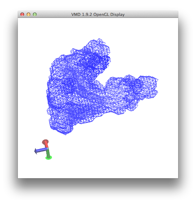
And the plot, once re-oriented for visual purposes, is shown below.
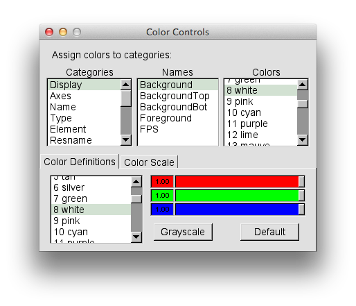
Your version will probably have a black background. To switch the color of the background to white, choose the "Colors" option from the "Graphics" pull-down tab. Select "Display" in the "Catagories" section, "Background" in the "Names" section, and "8 white" in the "Colors" section, as shown in the picture below.
At this point you are displaying the region of three-dimensional space for all structures that were accepted from the constrained Monomer Monte Carlo example.
In this section the original structure along with the accepted structures from the simulation will be loaded into a new molecule in the same VMD session described above.
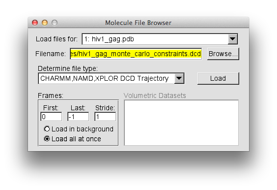
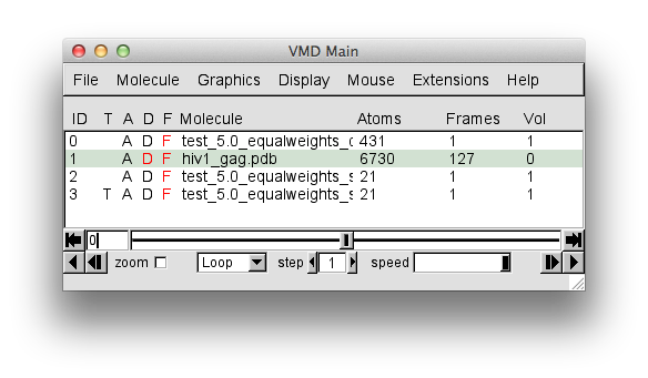
From "File" chose "New Molecule" and load the hiv1_gag.pdb file. Then, in the same "Molecule File Browser" load the trajectory from hiv1_gag_monte_carlo_constraints.dcd. Your "VMD Main Menu" and "Molecule File Browser" should look like the screen shots below.
NOTE It is faster to select "Load all at once" option in the "Molecule File Browser" when loading a large trajectory. This sidesteps the animation of each frame as the trajectory loads.
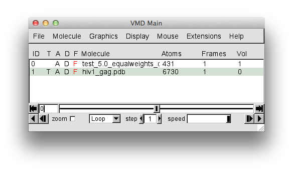
The trajectory contains 127 frames. The "hiv1_gag.pdb" entry in the "Molecule File Browser" will indicate that there are 128 frames loaded. This is because the PDB of the starting structure was loaded before the trajectory. That original structure may or may not have been accepted. So for completeness, this single frame should be removed.
NOTE VMD counts frames starting at 0, not 1.
To remove frame 0, the coordinates from the starting PDB file, select the "Delete Frames..." option from the "Molecule" pull-down tab. Then in the "Frame Selector" pop-up windown change the value of the "Last" frame from 127 to 0** as shown on the right side of the image below.
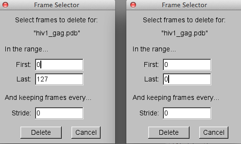
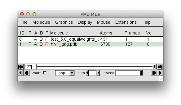
Then hit the "Delete" button to complete the task. The "VMD Main Menu" should now indicate that only 127 frames are in the "hiv1_gag.pdb"** molecule.
In the Open GL window, it may be difficult to see the protein structure. In the "Graphical Reprentations" window, select "VDW" in the "Drawing Method" option box. This will give you something similar to the view below.
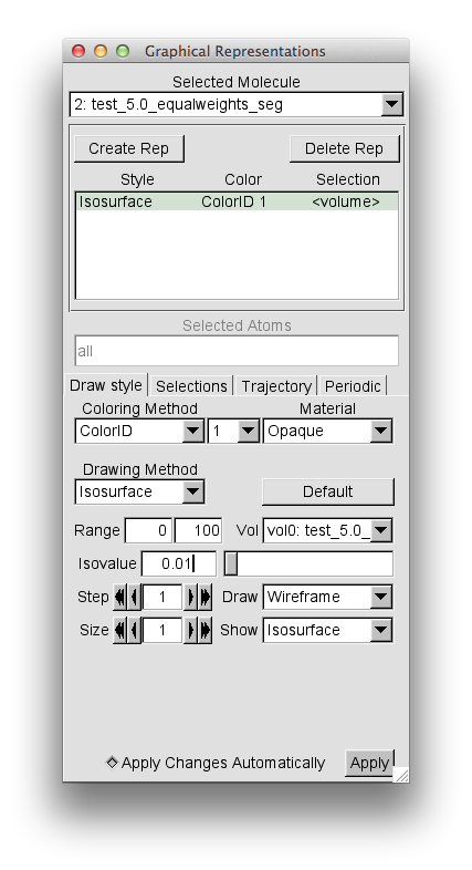
From "File" chose "New Molecule" and load the test_5.0_equalweights_segment_1_region_1.cube file. As described above, then select the "Graphical Reprentations" widget from "Reprentations" selection in the "Graphics" pull-down tab. Then, for the "Drawing Method" option choose "Isosurface". Then change the "Isovalue" from the default 0 to 0.01 and press return.
Then change the "Coloring Method" to "Color ID" and select 1 as the option.
This should give you the following window.
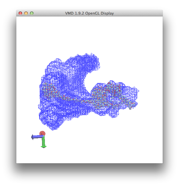
and a view in the OpenGL display similar to this
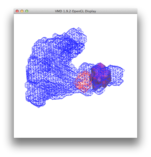
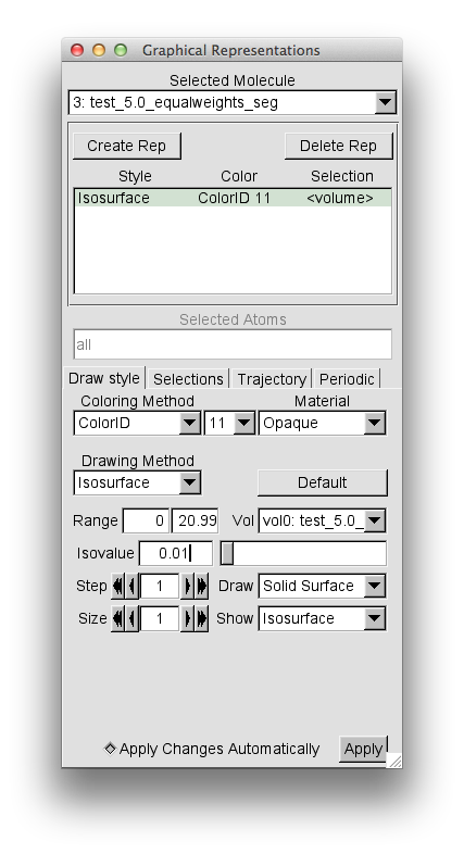
From "File" chose "New Molecule" and load the test_5.0_equalweights_segment_1_region_2.cube file. As described above, then select the "Graphical Reprentations" widget from "Reprentations" selection in the "Graphics" pull-down tab. Then, for the "Drawing Method" option choose "Isosurface". Then change the "Isovalue" from the default 0 to 0.01 and press return.
Then change the "Coloring Method" to "Color ID" and select 11 as the option.
This should give you the following window.
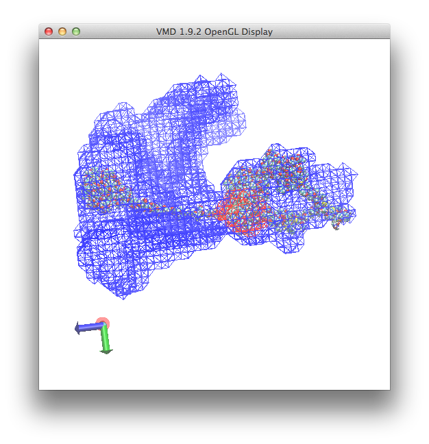
and a view in the OpenGL display similar to this
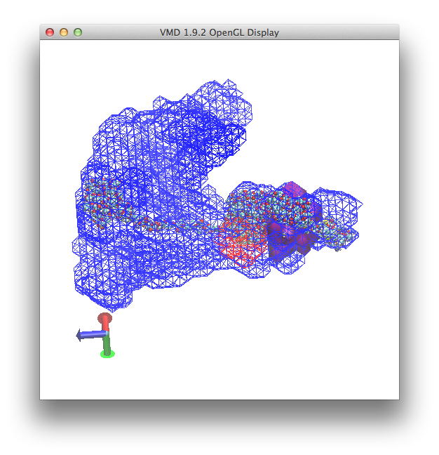
To obtain a final image similar to that shown in Density Plot example 1, merely toggle the "D" or display option for the "hiv1_gag.pdb" molecule as shown below.
To remove the axes label select "Axes" "off" from the "Display" pull-down tab. This will result in the final image.