Calculates small-angle neutron and X-ray scattering intensity curves from input all-atom structures.
The SasCalc module is accessible from the Calculate section of the main menu.
The purpose of the module is to calculate neutron and X-ray scattering profiles from a user supplied structure file using an exact all-atom expression for the scattering intensity in which the orientations of the q vectors are taken from a quasi-uniform spherical grid generated by the golden ratio. This "golden vector" method is currently configured to handle atomic trajectory input files (DCD or PDB).
The starting structure must be a complete structure without missing residues or atoms in order to obtain accurate scattering profiles. Atom and residue naming must be compatiable with those defined in the CHARMM force field See Notes on Starting Structures and Force Fields and PDB Scan for further details.
Different regions of the structure are specified using VMD selection syntax, i.e, all, chain, segname, index, resid, moltype, etc. See the documentation for VMD for further details.
The default input file format is DCD. For large numbers of frames we recommend saving your data in the DCD format (~seven fold smaller file size).
The program does not determine if the input parameters are adequate to converge the scattering profile over the desired range of q. This is the responsbilitiy of the user. However, the program does offer the option to calculate the scattering intensities using a "converged number of golden vectors" option in which the scattering profile is calculated several times using an increasing number of golden vectors until there is no difference between the calculated scattering curves to within a chosen tolerance (averaged over the entire scattering profile).
Even if only one structure is to be used to calculate a theoretical scttering curve, it still needs a reference structure even if the coordinates are in a PDB file.
More data points may not be mathematically justified. For SAS there is limited information content related to the size of the molecule measured in the experimental scattering data. 15 to 31 points are generally used. See BIOISIS for a theoretical and pratical reasoning regarding the number of points one should use.
The number of q-points, range of q, and the spacing of the q-points used to create interpolated data files MUST match the input settings that you use in this module to calculate SANS profiles if you wish to compare theoretical and experimental data (Chi-Square Filter).
The final range of q will be from 0 to a maximum q-value of (number of q-values - 1) * delta q, where delta q is the spacing between adjacent q-values entered by the user.
The calculated SAS profiles can be extracted using Extract Utilities or combined from multiple runs using Merge Utilities.
The recommended workflow is to first calculate the SAS intensity of a single structure file a few times using the "converged number of golden vectors" option. Note number of golden vectors needed to converge the scattering intensities to the desired tolerance, which is found in the output log files. This number should then be used in subsequent runs using the "fixed number of golden vectors" option.
This example calculates SANS profiles of a trajectory of 692 structures for the HIV-1 gag protein. The number of q values and the maximum q value were chosen to match previously-interpolated data contained in the sans_data.dat file.
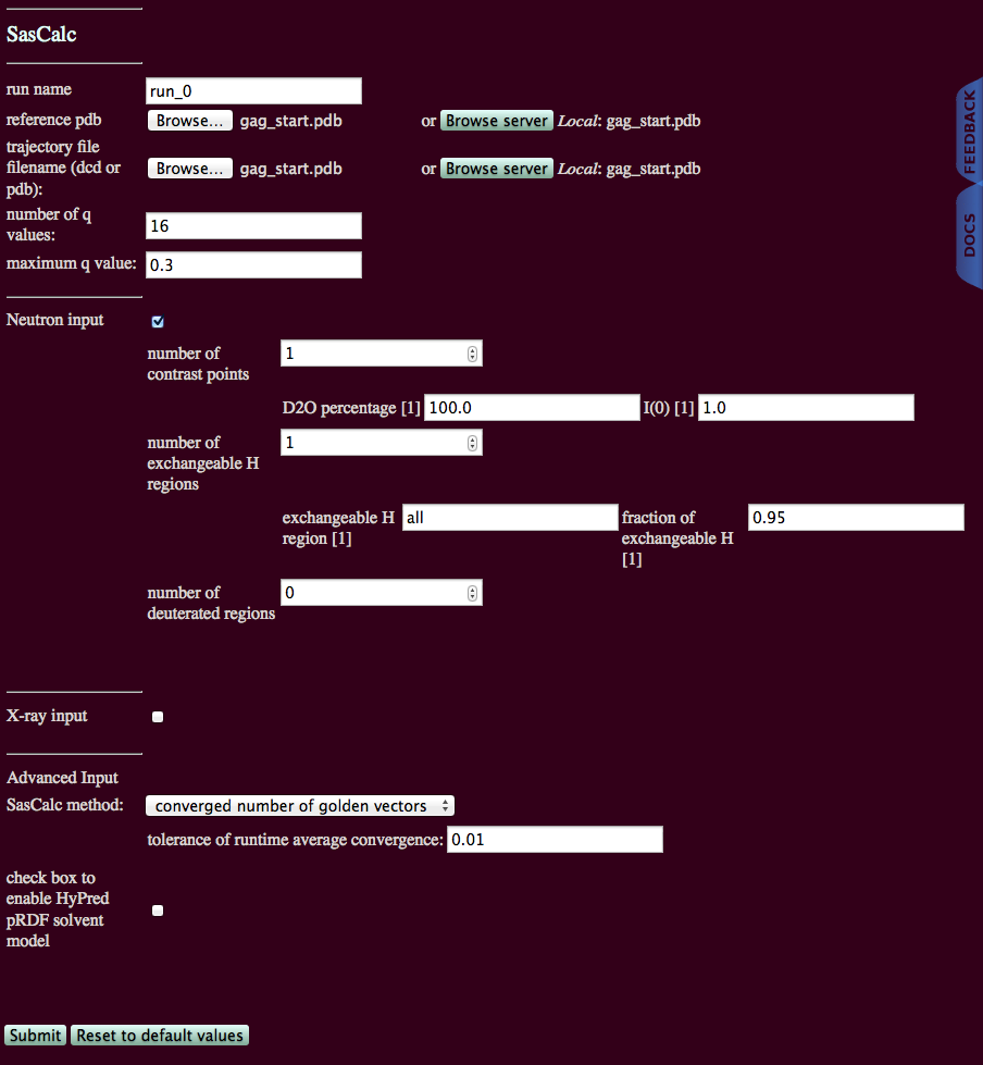
The module is first run using the "converged number of golden vectors" option on just one structure.
run name: user defined name of folder that will contain the results.
reference pdb: PDB file with naming information for coordinates that will be extracted
trajectory file filename (dcd or pdb): DCD or PDB file with coordinates that will be used to calculate scattering profile(s).
number of q values: The number of individual q-points for which I(q) is calculated, including q=0.
maximum q value: The maximum value to calculate I(q).
Neutron input: Check box to calculate SANS intensity profiles.
X-ray input: Check box to calculate SAXS intensity profiles. (Not used in this example.)
NOTE: Both Neutron input and X-ray input boxes can be checked at the same time.
SasCalc method: Choose fixed number of golden vectors or converged number of golden vectors from the pull-down menu (default is fixed number of golden vectors).
check box to enable HyPred pRDF solvent model: Not yet implemented.
Not yet available:
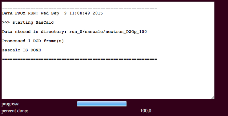
The output will indicate the number of processed frames and the location of the scattering profiles.
Results will be written to a new directory within the given "run name". For example, in the figure it is noted that the calculated scattering intensities and associated log and information files are found in a subdirectory named for the type of radiation chosen and the percentage of D2O, if applicable. In this case, files are written to:
./run_0/sascalc/neutron_D2Op_100/
None
input files
output files
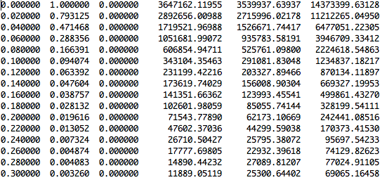
The first three columns in the scattering intensity file contain q, I(q) normalized to the chosen I(0) value, and the error in I(q). The latter is just a column of zeros if only one iteration of SasCalc is performed. The last three columns in the file contain the unnormalized I(q) values for the vacuum - solvent scattering, the vacuum scattering alone and the solvent scattering alone.
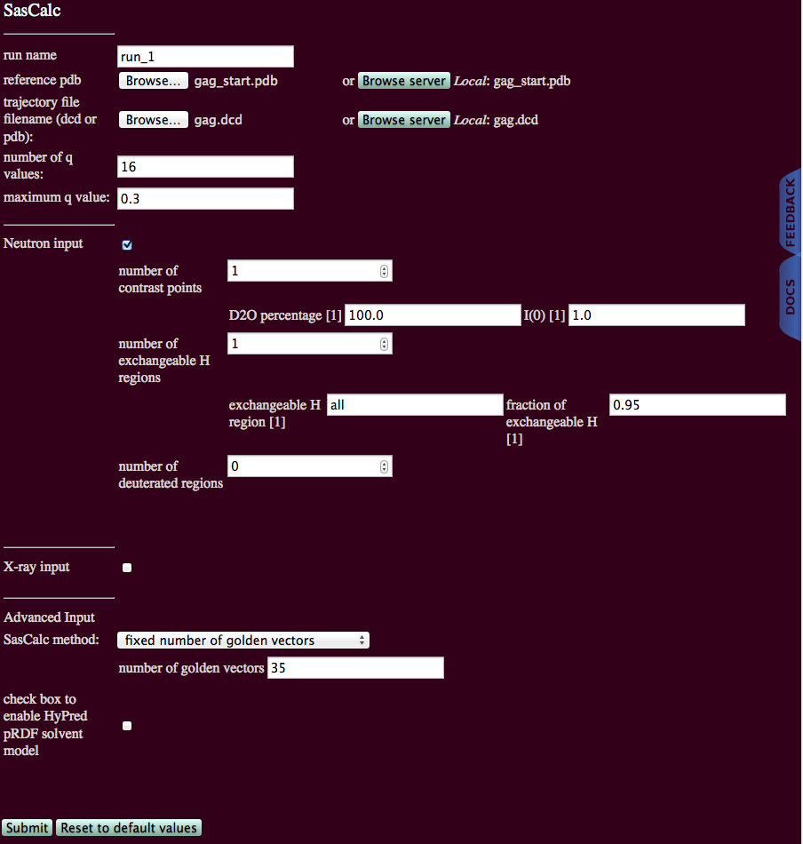
The information in the run000001.log file indicates that 35 golden vectors were needed to converge the scattering profile to the chosen tolerance of 0.01. Now, the module can be run on the entire trajectory of 692 structures using the "fixed number of golden vectors" option with 35 golden vectors.
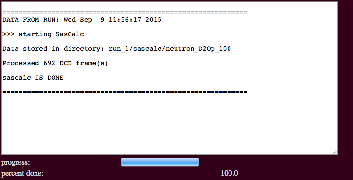
The output will indicate the number of processed frames and the location of the scattering profiles.
./run_1/sascalc/neutron_D2Op_100/
None
input files
output files
scattering profiles, log files and other information files are provided as a compressed archive
This example calculates SAXS profiles of a trajectory of 692 structures for the HIV-1 gag protein over a wider q-range than for the SANS examples above.
Since the SAXS intensities will be calculated over a wider q-range, it cannot be assumed that the same number of golden vectors that was used for the SANS intensities will converge the SAXS intensities to the same tolerance! Thus, an initial run on one structure was performed using the "converged number of golden vectors" option. The results revealed that 41 golden vectors are needed to converge the SAXS scattering profiles to a tolerance of 0.01. This example will use the "fixed number of golden vectors option" with 41 golden vectors to calculate the SAXS scattering profiles.
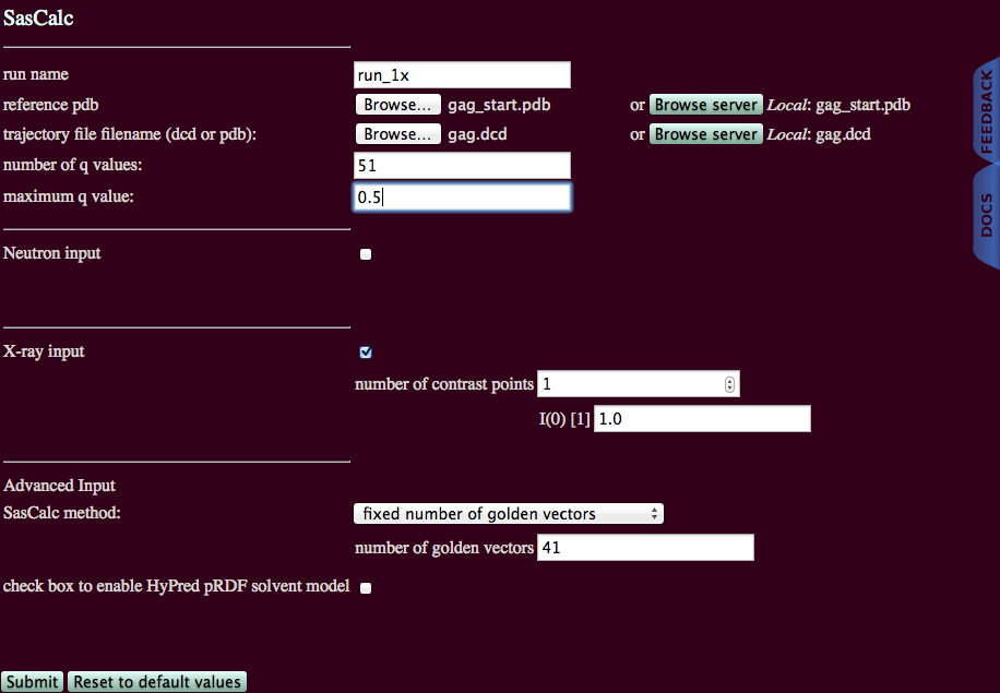
NOTE: The HyPred pRDF solvent model should be used here once it has been implemented.
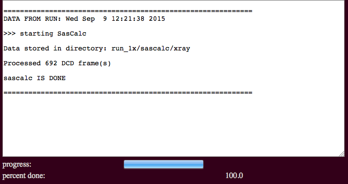
The output will indicate the number of processed frames and the location of the scattering profiles.
./run_1x/sascalc/xray/
None
input files
output files
scattering profiles, log files and other information files are provided as a compressed archive
This example calculates SANS profiles of a trajectory of 622 structures for a protein-RNA complex.
An initial run on one structure using the "converged number of golden vectors" option for several different contrasts revealed that 41 golden vectors are needed to converge the scattering profiles to a tolerance of 0.01. This example will use the "fixed number of golden vectors option" with 41 golden vectors to calculate the scattering profiles at four different contrast points.
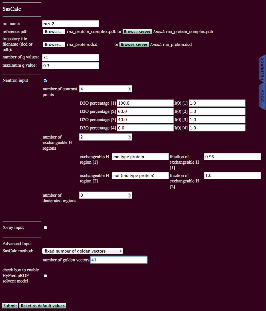
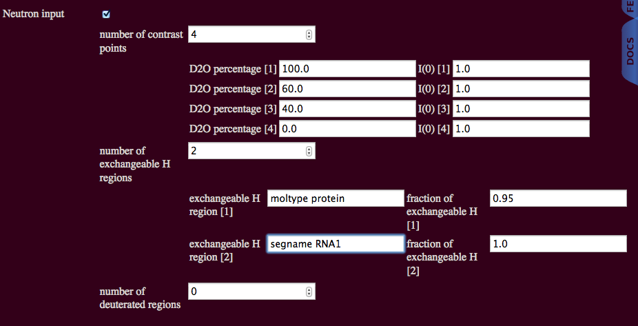
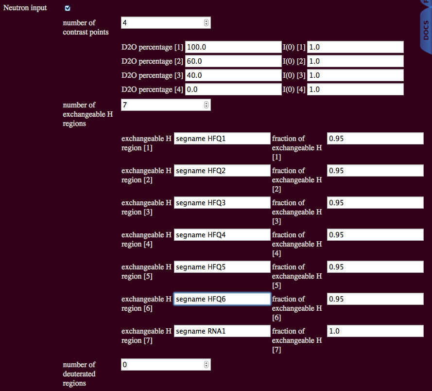
Protein and RNA have different H-D exchange rates. We are assuming that 95% of all exchangeable H atoms are exchanging for proteins and 100% for RNA. The protein consists of 6 chains and the PDB file also designates 6 segment names. The RNA is a single chain and has a single segment name. All of the protein segments can be selected at once using the syntax below. The RNA segment can be selected by excluding protein using the syntax below.
Neither the protein nor the RNA is deuterated. So, we can have no deuterated regions.
The RNA segment name can be used explicitly for the RNA part of the complex.
The protein and RNA segment names can be used explicitly. Chain names can be used in a similar manner.
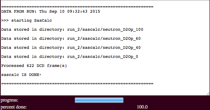
The output will indicate the number of processed frames and the location of the scattering profiles.
./run_2/sascalc/neutron_D2Op_100/
./run_2/sascalc/neutron_D2Op_60/
./run_2/sascalc/neutron_D2Op_40/
./run_2/sascalc/neutron_D2Op_0/

These intensity plots scaled to I(0) = 1.0 show how the scattering profiles change shape as a function of contrast. The profiles were calculated using the "converged number of golden vectors" option with a tolerance of 0.01 (lines) and the "fixed number of golden vectors" option with the number of golden vectors set to 41 (points). A distinct interaction peak is present due to intra-particle correlations at 60% D2O. Unfortunately, 60% D2O is very close to both the match point of the RNA (63% D2O) and that of the entire complex (56% D2O). Thus, the scattering intensity is too small to be measured at this contrast and these intra-particle correlations can not be observed in practice. Match points and absolute scattering intensities can be calculated as a function of contrast for a given concentration of the complex using Contrast Calculator.
input files
output files
scattering profiles, log files and other information files are provided as a compressed archive
This example calculates SANS profiles of a trajectory of 600 structures a complex consisting of one deuterated and one non-deuterated subunit. In the deuterated subunit, 50% of the non-exchangeable hydrogen atoms have been replaced with deuterium.
An initial run on one structure using the "converged number of golden vectors" option for several different contrasts revealed that 33 golden vectors are needed to converge the scattering profiles to a tolerance of 0.01. This example will use the "fixed number of golden vectors option" with 35 golden vectors to calculate the scattering profiles at four different contrast points.
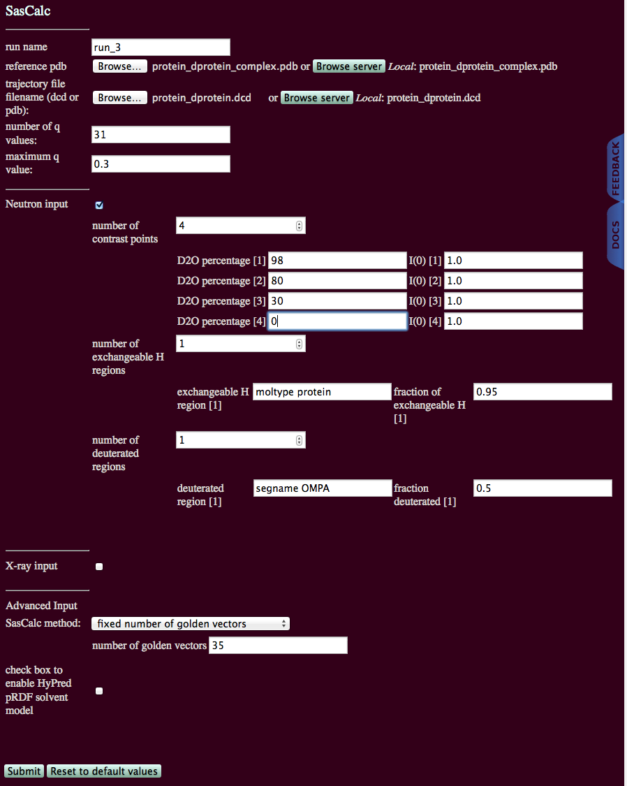
We are assuming that 95% of all exchangeable H atoms are exchanging for both protein subunits. The deuterated subunit is designated with the segment name OMPA and the non-deuterated protein has 3 segments designated SKP1, SKP2 and SKP3. However, all have the same exchange rate, so there is only one exchangeable H region.
Since one of the designated segments is deuterated we have one deuterated region for which the deuteration fraction must be specified:
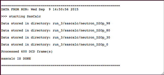
The output will indicate the number of processed frames and the location of the scattering profiles.
./run_3/sascalc/neutron_D2Op_98/
./run_3/sascalc/neutron_D2Op_80/
./run_3/sascalc/neutron_D2Op_30/
./run_3/sascalc/neutron_D2Op_0/
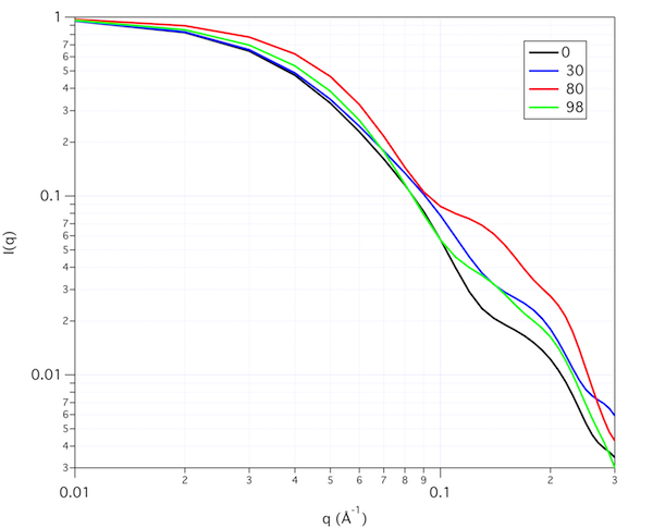
These intensity plots scaled to I(0) = 1.0 show how the scattering profiles change shape as a function of contrast. The profiles were calculated using the "converged number of golden vectors" option with a tolerance of 0.01.
input files
output files
scattering profiles, log files and other information files are provided as a compressed archive
HyPred pRDF solvent model is not yet implemented.
Rapid and accurate calculation of small-angle scattering profiles using the golden ratio M.C. Watson, J.E. Curtis, J. Appl. Crystallogr. 46, 1171-1177 (2013)). BIBTeX, EndNote, Plain Text
SASSIE: A program to study intrinsically disordered biological molecules and macromolecular ensembles using experimental scattering restraints J. E. Curtis, S. Raghunandan, H. Nanda, S. Krueger, Comp. Phys. Comm. 183, 382-389 (2012). BIBTeX, EndNote, Plain Text